Method

Overview

1. Signal Processing - Broadband Characteristic Function Calculation

Exctracting non-stationary frequency-dependent statistical features of the recorded seismic signals.

Higher-Order Statistics (HOS) CFs

Estimating CF of the raw record by extracting information on the statistical variations of the signal. Suitable for enhansing and extracting short transient signals e.g., local earthquakes, phase arrivals from distant events, and other short transients assosiated to low frequency earthquakes and vulcanic earthquakes. HOS perform well in the conditions of low signal-to-noise ratio.

HOS of a probability distribution for a random variable \(X\) are defined by the standardized moment:

\[S_n = \frac {E \left[ \left( X - \mu \right)^n \right]} {\left( E \left[ \left( X - \mu \right)^2 \right] \right)^ {n/2}} = \frac{m_n}{m_2^{n/2}}\]

where \(E\left[\cdot\right]\) is the expectation operator, \(\mu = E\left[X\right]\) is the mean, \(m_2 = \sigma^2\) is the variance (second moment), and \(m_n\) is the \(n^{th}\) central moment.

Kurtosis, is the HOS of the \(4^{th}\) order. It is defined as a \(4^{th}\) moment about the mean normalized by the square of the \(2^{nd}\) moment (variance) - \(S_4 = m_4/m_2^2\) . Although, HOS of higher orders can be equally used, in his version of the program we limit the calculation of HOS CFs to kurtosis.

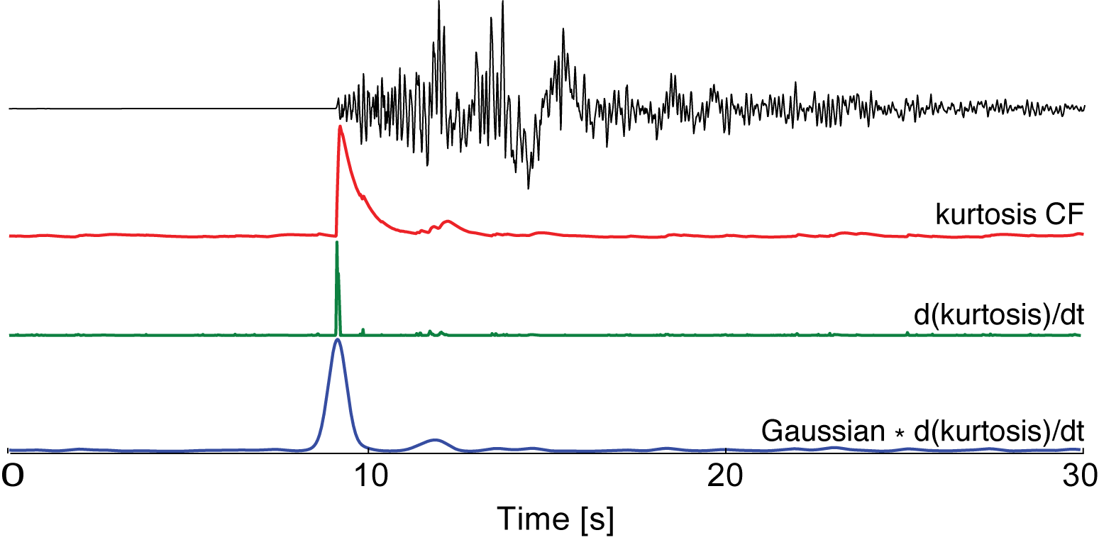
Calculation of kurtosis for a discrete signal \(u\left(t\right)\) (seismic record) is clasically performed in a sliding window. This can be computationally expensive. To improve the computational performance we implemented a recursive scheme based on formulation of the exponential moving average. Such scheme provides an efficient way for accumulating time-averaged statistics. The recursive formula for exponential moving average \(\hat{\mu}\left(t\right)\) of signal \(u\left(t\right)\) is defined as:

\[\hat{\mu}\left(t_i\right)= C\times u\left(t_i\right)+\left(1-C\right) \times \hat{\mu}\left(t_{i-1}\right)\]

where \(u\left(t_i\right)\) is the \(i\)-th sample of the signal, \(\hat{\mu}\left(t_{i-1}\right)\) previous estimate of the average, and \(C\) is the decay constant (\(0\leq 1-C \leq 1\)). Directly extending the above definition to the estimates of the \(2^{nd}\) and \(4^{th}\) cantral moments, and using the definition of HOS we obtain the following recursive expression for the kurtosis CF:

\[CF_{HOS} \left(t_i\right) \equiv\ \hat{S}_4\left(t_i\right) = \frac {C \times \left[u\left(t_i\right) - \hat{\mu}\left(t_{i-1} \right)\right]^4 +\left( 1-C \right) \times \hat{m}_4\left(t_{i-1}\right)} {\left( C \times \left[u\left(t_i\right) - \hat{\mu}\left(t_{i-1} \right)\right]^2 +\left( 1-C \right) \times \hat{m}_2\left(t_{i-1}\right)\right)^2}\]

For a more general case of the \(n^{th}\) order HOS replace \(4\) with \(n\) in the above formula. Currently code is tested for orders \(n = 4, 6, 8\)

An example of the recursive kurtosis CF calculated on a seismogram of a regional earthquake is shown below.

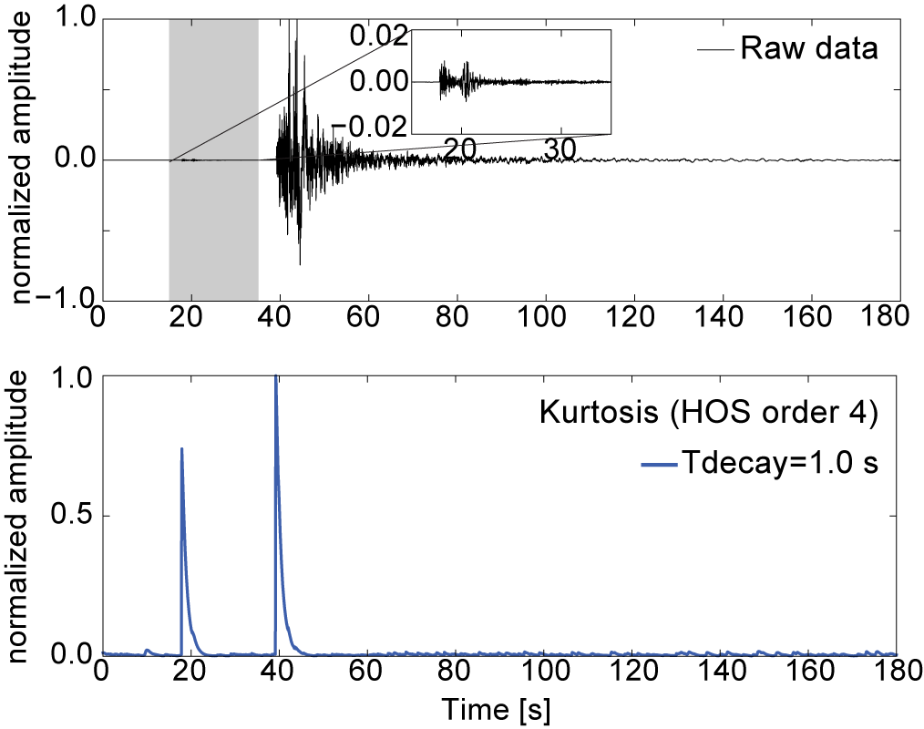
The decay constant \(C\) can be as seen as a smoothing factor, defining how fast the memory of older data-points will be discarded. It is expressed as \(C = \frac{\Delta T}{T_{decay}}\) where \(\Delta T\) is sampling rate of the data and \(T_{decay}\) represents the time-length of the averaging scale. Effect of different values of \(C\) constant on the final CF is shown in the following figure.

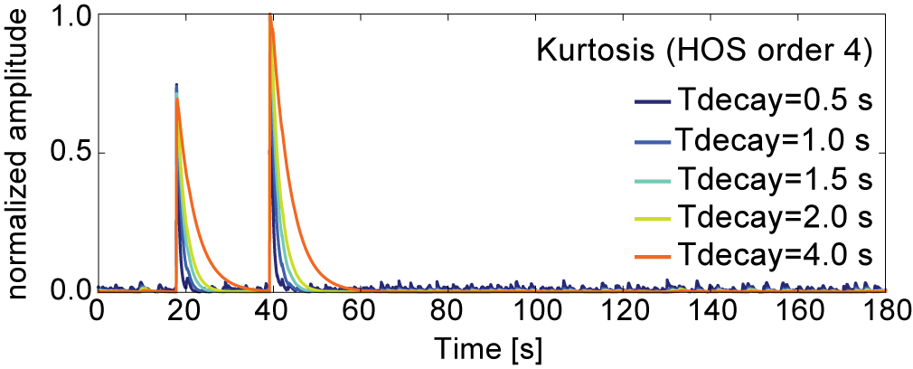
Decay constant \(C\) should be set separately for each particular case study, through a preliminary testing step. The actual value of this parameter is defined by selecting \(T_{decay}\) (in seconds) in the program’s control file. The parameter is further transformed into the decay constant, using the sampling rate of the data.

Envelope CFs

Characterization of signal based on the amplitude or energy modulation - energy envelope that can be applied to signals associated to sources characterized by slow energy transients, lasting several tens of seconds e.g., tectonic tremors. The relative timing of localized energy transients can be used to detect and locate a tremor source.

The root-mean-square (RMS) envelope CF function is defined as:

\[CF_{env} \left( t_i \right) \equiv RMS(t_i) = \sqrt {\frac{\sideset{}{_{i=1}^M}\sum u(t_i)^2}{M-1}}\]

Following the same idea of recursive implementation, we define the recursive envelope CF as a single component recursive RMS envelope of the recorded signal \(u\left(t_i\right)\) using following expression:

\[CF_{env}( t_i ) \equiv \widehat{RMS}(t_i) = \sqrt{C \times u^2(t_i) + (1-C) \times\left[\widehat{RMS}(t_{i-1}) \right]^2 }\]

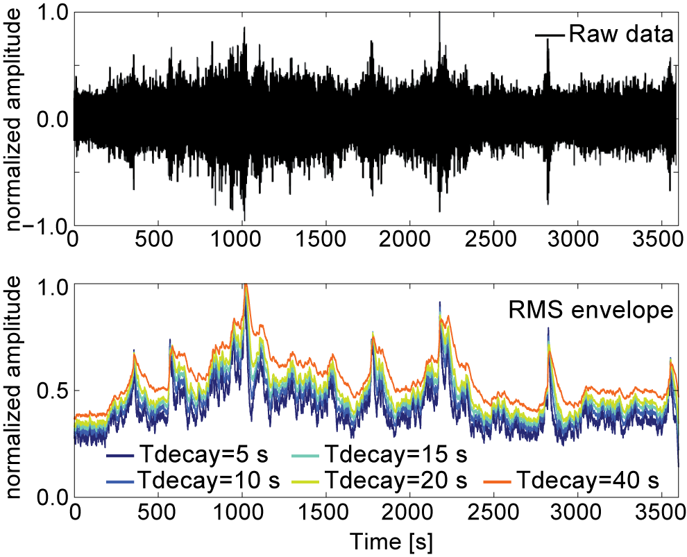
Similarly to the recursive kurtosis CF, parameter to be set for the calculation is \(T_{decay}\) in seconds, from which the decay constant is calculated as \(C = \frac{\Delta T}{T_{decay}}\).

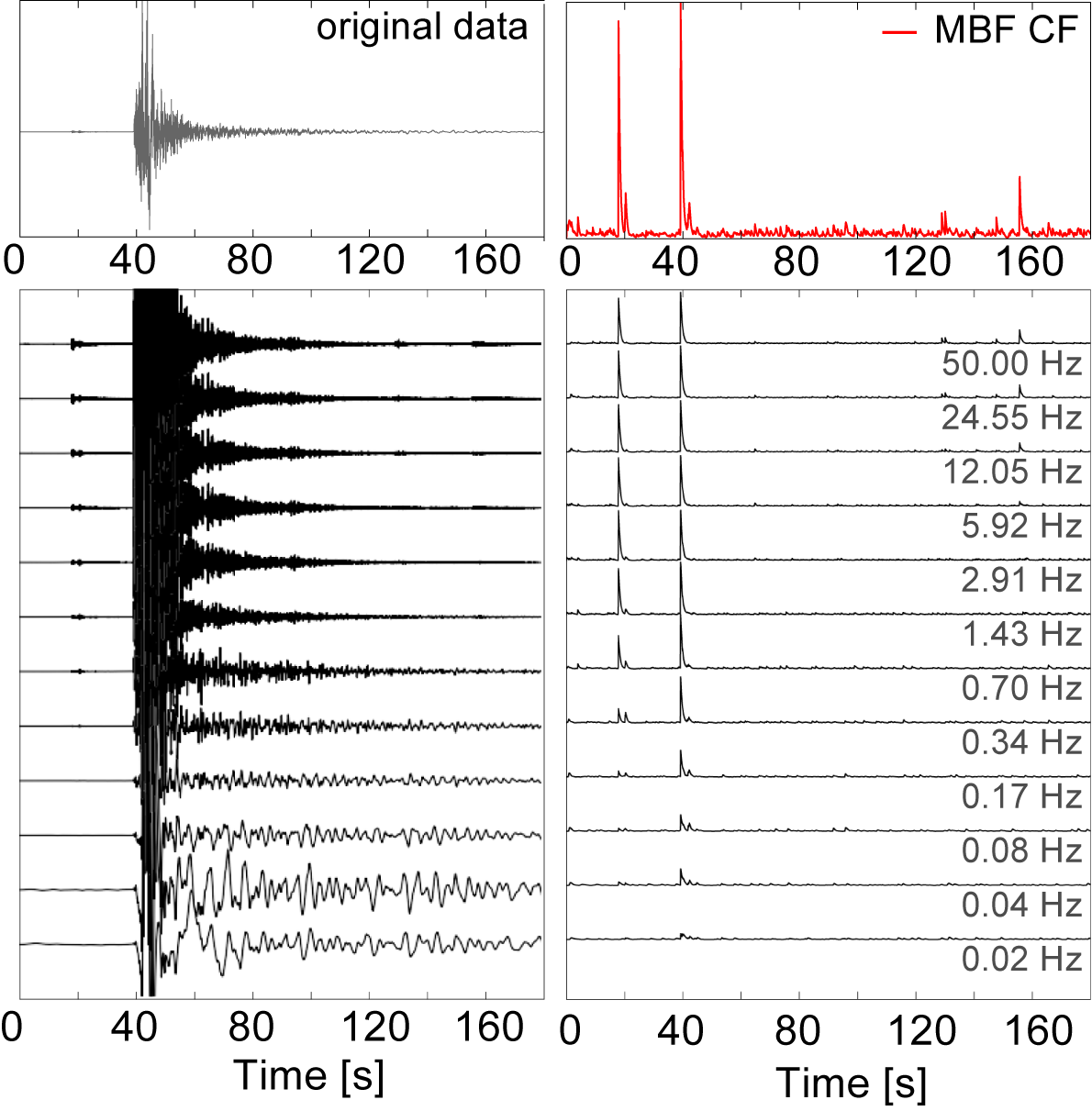
Time-Frequency Analyasis: Multi-Band Filter

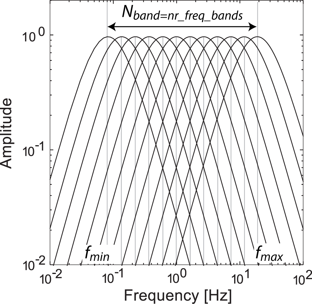
The Multi-Band Filter (MBF) algorithm performs a time-frequency decomposition of the signal by producing a set of band-pass filtered time series with different central periods. Implemented MBF scheme follows the recursive multi-band filtering scheme of FilterPicker algorithm by Lomax et al. (2012). MBF analysis is performed by running the original record through a predefined bank of narrow band-pass filters covering the interval \(\left[ f_{min},f_{max} \right]\), and having \(n = \left\{0,...,N_{band}\right\}\) central frequencies (either linearly or logarithmically spaced). On practice, filtering is implemented through a cascade of two simple low-pass and high-pass, one-pole recursive filters. This is equivalent to a two-pole band-pass filter. Below is an illustration of such a filter-bank:

A frequency-dependent CFs (\(CF(t,f_n)\)) calculated by running the kurtosis/envelope recursive estimations for each of the filtered signals. This yields a time-frequency dependent representation of the signal’s characteristics.

\[CF^{TF}(t)=\max\limits_f CF(t,f), \quad f\in [f_{min},f_{max}]\]

Generalized Characteristic Function

\[\begin{split}CF(t) = \begin {cases} \sideset{}{_{HOS}^+}{\dot{CF}}(t) \ast e^{t^2/4\sigma^2} & \quad \text{if } CF\text{_}type \text{ is } kurtosis \\ \\ CF_{env}(t) & \quad \text{if } CF\text{_}type \text{ is } envelope \\ \end{cases}\end{split}\]

2. Detection and Location Scheme

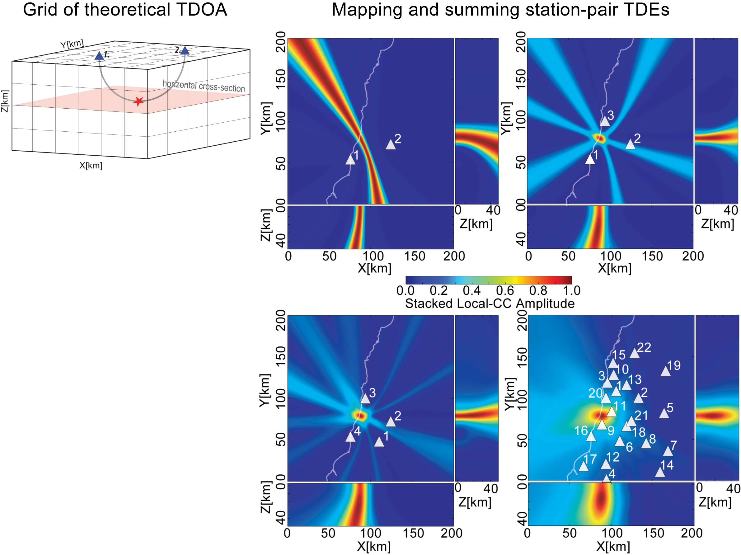
Detection and location is based on stacking Spatial Likelihood Functions (SLFs) according to the theoretical 3-D travel-time grids. SLF are corresponding to the station-pair time-delay estimate functions. The procedure of stacking the projected SLF functions can be viewed as space-time imaging procedure.

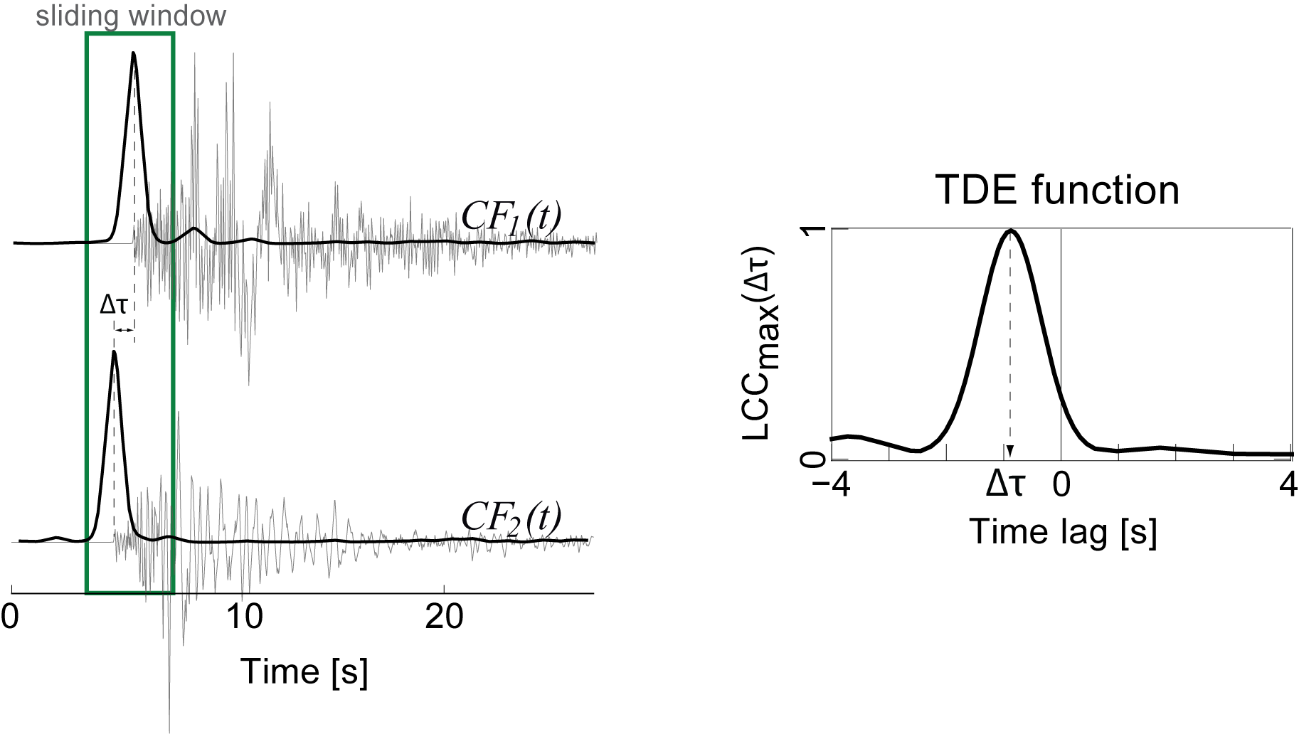
Stations-pair Time Delay Estimate (TDE) Functions

Corresponds to maximum local cross-correlation function (see Poiata et al., 2016 for details) calculated in a given time window.

Space-Time Imaging

Performs projection (mapping) and stacking of staion-pairs TDE according to the theoretical 3-D travel-times calculated for a given velocity model:

Detection and Location

Performed for each position of a sliding time window on a final imaging function (summary SLF) if its maximum value exceeds the selected threshold value.

Analysing continuous data