Tests and Examples
The code is provided with examples, for testing that all the things are installed and running ok, and also allowing to play around with the parameters. This may help to understand better how the things a working.
Download file examples.zip. After
uncompressing it you will get folder examples/ containing all the data
(seismograms and theoretical travel-time grids) that you will need to run the
examples.
Detection and location
Use config file BT_ChileExample.conf. Check that folder with examples is in
the same folder with the main code and configuration file, otherwise change the
path to data_dir and grid_dir .
Run the detection and location code:
$ btbb examples/BT_ChileExample.conf

use of var time window for location: False
Number of traces in stream =  22
Number of time windows =  1
frequencies for filtering in (Hz): [  2.00000000e-02   3.01583209e-02   4.54762160e-02   6.85743157e-02
1.03404311e-01   1.55925020e-01   2.35121839e-01   3.54543993e-01
5.34622576e-01   8.06165961e-01   1.21563059e+00   1.83306887e+00
2.76411396e+00   4.16805178e+00   6.28507216e+00   9.47736116e+00
1.42910650e+01   2.15497261e+01   3.24951778e+01   4.90000000e+01]
starting BPmodule
Running on 1 thread
22
20100401_1253A X 5.0 Y 33.0 Z 16.0 MaxStack 0.858 Ntraces 22 BEG 33.0 END 53.0  LAT -34.70242 LON -72.04541 T_ORIG 2010-04-01T12:53:05.343609Z
You should get following outputs written in the directory defined in out_dir:
10040112_20fq0.0_49.0hz_1.050.00.117.0_kurtosis_HHZ_P_trig0.7_FIG2.png0040112_20fq0.0_49.0hz_1.050.00.117.0_kurtosis_HHZ_P_trig0.7_OUT2.dat10040112_t0033.0s_0.0_49.0_fig.png
The image files should look like:
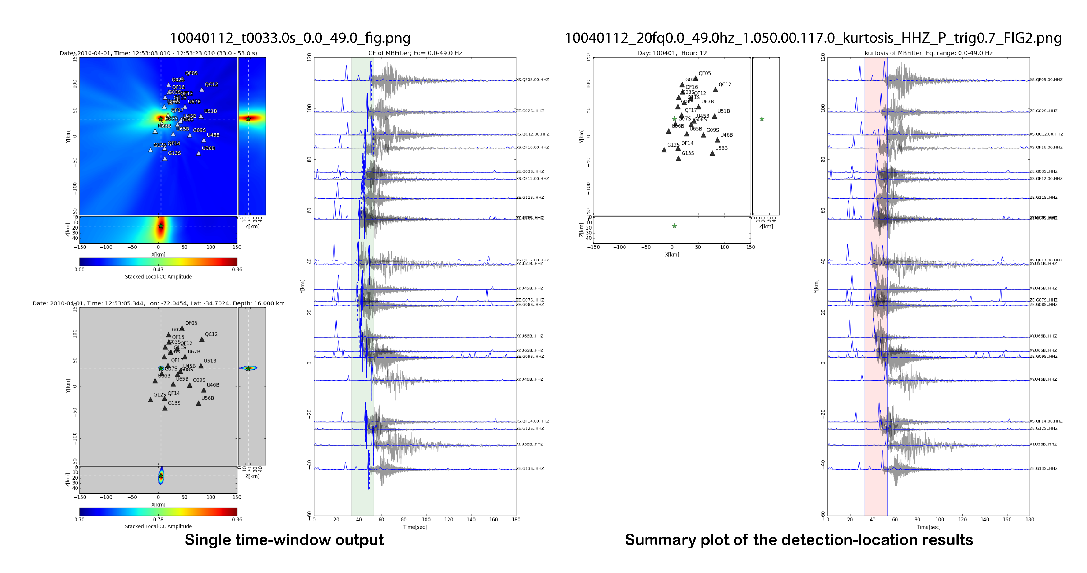
0040112_20fq0.0_49.0hz_1.050.00.117.0_kurtosis_HHZ_P_trig0.7_OUT2.dat - summary text file. It will have full information on the location of the triggered event and arrival times of the phase to the stations:
20100401_1253A X 5.0 Y 33.0 Z 16.0 MaxStack 0.858 Ntraces 22 BEG 33.0 END 53.0  LAT -34.70242 LON -72.04541 T_ORIG 2010-04-01T12:53:05.343609Z
 sta G02S  Ph P  TT 12.08  PT 12.17
 sta G03S  Ph P  TT 7.95  PT 8.14
 sta G06S  Ph P  TT 5.09  PT 5.07
 sta G07S  Ph P  TT 3.23  PT 2.92
 sta G08S  Ph P  TT 6.49  PT 6.86
 sta G09S  Ph P  TT 11.47  PT 11.53
 sta G11S  Ph P  TT 7.02  PT 7.29
 sta G12S  Ph P  TT 11.33  PT 11.60
 sta G13S  Ph P  TT 13.53  PT 13.40
 sta QC12  Ph P  TT 17.12  PT 16.16
 sta QF05  Ph P  TT 15.63  PT 15.06
 sta QF12  Ph P  TT 9.20  PT 9.08
 sta QF14  Ph P  TT 10.38  PT 10.48
 sta QF16  Ph P  TT 9.81  PT 9.92
 sta QF17  Ph P  TT 3.85  PT 3.81
 sta U45B  Ph P  TT 7.14  PT 7.48
 sta U46B  Ph P  TT 16.21  PT 16.28
 sta U51B  Ph P  TT 13.76  PT 13.59
 sta U56B  Ph P  TT 17.35  PT 17.13
 sta U65B  Ph P  TT 7.10  PT 7.52
 sta U66B  Ph P  TT 5.32  PT 5.59
 sta U67B  Ph P  TT 9.42  PT 9.40
Signal processing: MBF characteristic functions
Run the MBF signal processing example for a defined filter bank and Kurtosis CF:
$ mbf_plot examples/MBF_ChileExample.conf
This code can be useful to understand how the MBF filtering and CF calculation works, and for adjusting the signal processing parameters for the data.
Output should look like:
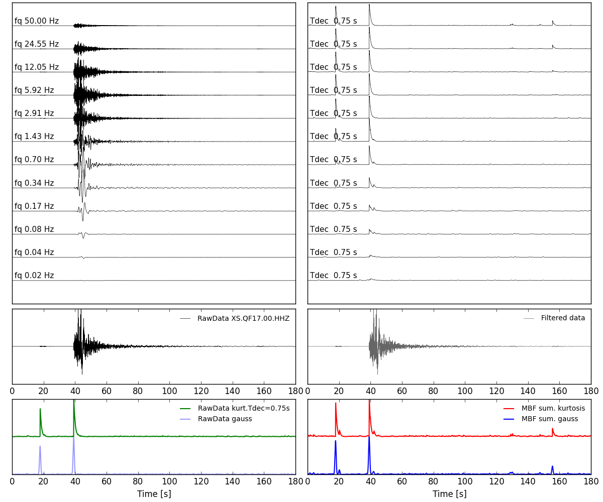
mbf_plot is useful for deciding most appropriate signal-processing
parameters for your data.